Question: Given the aroma/bitterness/etc of a cup of coffee, can we predict if it will be a ‘good’ cup of coffee as rated by professional coffee tasters?
Check out the Jupyter Notebook to follow along.
We’ll bring in the data, do preliminary exploration, transform it for analysis, separate it into training/test sets, determine which model results in the highest accuracy predictions, and predict the rating a new cup of coffee might receive.
Info from The Coffee Institute, data scraped by James LeDoux.
Let’s start with our initial imports. This will bring in everything we’ll need for the project, including ways to manipulate data (pandas), visualize data (matplotlib), and do ML analysis (sklearn)
#importing
##data tools
import pandas as pd
pd.set_option('display.max_columns', 500)
import matplotlib.pyplot as plt
import matplotlib.colors as mcolors
##ML tools
from sklearn.ensemble import RandomForestClassifier
from sklearn import svm
from sklearn.svm import SVC
from sklearn.neural_network import MLPClassifier
from sklearn.metrics import confusion_matrix, classification_report
from sklearn.preprocessing import StandardScaler, LabelEncoder
from sklearn.model_selection import train_test_split
%matplotlib inline
Next let’s get the data and take a quick look at it.
coffeeRaw = pd.read_csv('arabica_data_cleaned.csv')coffeeRaw.head()| Unnamed: 0 | Species | Owner | Country.of.Origin | Farm.Name | Lot.Number | Mill | ICO.Number | Company | Altitude | Region | Producer | Number.of.Bags | Bag.Weight | In.Country.Partner | Harvest.Year | Grading.Date | Owner.1 | Variety | Processing.Method | Aroma | Flavor | Aftertaste | Acidity | Body | Balance | Uniformity | Clean.Cup | Sweetness | Cupper.Points | Total.Cup.Points | Moisture | Category.One.Defects | Quakers | Color | Category.Two.Defects | Expiration | Certification.Body | Certification.Address | Certification.Contact | unit_of_measurement | altitude_low_meters | altitude_high_meters | altitude_mean_meters | |
|---|---|---|---|---|---|---|---|---|---|---|---|---|---|---|---|---|---|---|---|---|---|---|---|---|---|---|---|---|---|---|---|---|---|---|---|---|---|---|---|---|---|---|---|---|
| 0 | 1 | Arabica | metad plc | Ethiopia | metad plc | NaN | metad plc | 2014/2015 | metad agricultural developmet plc | 1950-2200 | guji-hambela | METAD PLC | 300 | 60 kg | METAD Agricultural Development plc | 2014 | April 4th, 2015 | metad plc | NaN | Washed / Wet | 8.67 | 8.83 | 8.67 | 8.75 | 8.50 | 8.42 | 10.0 | 10.0 | 10.0 | 8.75 | 90.58 | 0.12 | 0 | 0.0 | Green | 0 | April 3rd, 2016 | METAD Agricultural Development plc | 309fcf77415a3661ae83e027f7e5f05dad786e44 | 19fef5a731de2db57d16da10287413f5f99bc2dd | m | 1950.0 | 2200.0 | 2075.0 |
| 1 | 2 | Arabica | metad plc | Ethiopia | metad plc | NaN | metad plc | 2014/2015 | metad agricultural developmet plc | 1950-2200 | guji-hambela | METAD PLC | 300 | 60 kg | METAD Agricultural Development plc | 2014 | April 4th, 2015 | metad plc | Other | Washed / Wet | 8.75 | 8.67 | 8.50 | 8.58 | 8.42 | 8.42 | 10.0 | 10.0 | 10.0 | 8.58 | 89.92 | 0.12 | 0 | 0.0 | Green | 1 | April 3rd, 2016 | METAD Agricultural Development plc | 309fcf77415a3661ae83e027f7e5f05dad786e44 | 19fef5a731de2db57d16da10287413f5f99bc2dd | m | 1950.0 | 2200.0 | 2075.0 |
| 2 | 3 | Arabica | grounds for health admin | Guatemala | san marcos barrancas "san cristobal cuch | NaN | NaN | NaN | NaN | 1600 - 1800 m | NaN | NaN | 5 | 1 | Specialty Coffee Association | NaN | May 31st, 2010 | Grounds for Health Admin | Bourbon | NaN | 8.42 | 8.50 | 8.42 | 8.42 | 8.33 | 8.42 | 10.0 | 10.0 | 10.0 | 9.25 | 89.75 | 0.00 | 0 | 0.0 | NaN | 0 | May 31st, 2011 | Specialty Coffee Association | 36d0d00a3724338ba7937c52a378d085f2172daa | 0878a7d4b9d35ddbf0fe2ce69a2062cceb45a660 | m | 1600.0 | 1800.0 | 1700.0 |
| 3 | 4 | Arabica | yidnekachew dabessa | Ethiopia | yidnekachew dabessa coffee plantation | NaN | wolensu | NaN | yidnekachew debessa coffee plantation | 1800-2200 | oromia | Yidnekachew Dabessa Coffee Plantation | 320 | 60 kg | METAD Agricultural Development plc | 2014 | March 26th, 2015 | Yidnekachew Dabessa | NaN | Natural / Dry | 8.17 | 8.58 | 8.42 | 8.42 | 8.50 | 8.25 | 10.0 | 10.0 | 10.0 | 8.67 | 89.00 | 0.11 | 0 | 0.0 | Green | 2 | March 25th, 2016 | METAD Agricultural Development plc | 309fcf77415a3661ae83e027f7e5f05dad786e44 | 19fef5a731de2db57d16da10287413f5f99bc2dd | m | 1800.0 | 2200.0 | 2000.0 |
| 4 | 5 | Arabica | metad plc | Ethiopia | metad plc | NaN | metad plc | 2014/2015 | metad agricultural developmet plc | 1950-2200 | guji-hambela | METAD PLC | 300 | 60 kg | METAD Agricultural Development plc | 2014 | April 4th, 2015 | metad plc | Other | Washed / Wet | 8.25 | 8.50 | 8.25 | 8.50 | 8.42 | 8.33 | 10.0 | 10.0 | 10.0 | 8.58 | 88.83 | 0.12 | 0 | 0.0 | Green | 2 | April 3rd, 2016 | METAD Agricultural Development plc | 309fcf77415a3661ae83e027f7e5f05dad786e44 | 19fef5a731de2db57d16da10287413f5f99bc2dd | m | 1950.0 | 2200.0 | 2075.0 |
Ok. That’s a lot of info, far more than we need really. Remember, our goal is to build something that can predict a value using only information we might have about a cup of coffee right in front of us. We won’t know the elevation, processing method, etc. So let’s trim this down to a more useful dataset..
coffee = coffeeRaw[['Aroma','Flavor', 'Aftertaste', 'Acidity', 'Body', 'Balance',
                     'Total.Cup.Points']].copy()
coffee.head()| Aroma | Flavor | Aftertaste | Acidity | Body | Balance | Total.Cup.Points | |
|---|---|---|---|---|---|---|---|
| 0 | 8.67 | 8.83 | 8.67 | 8.75 | 8.50 | 8.42 | 90.58 |
| 1 | 8.75 | 8.67 | 8.50 | 8.58 | 8.42 | 8.42 | 89.92 |
| 2 | 8.42 | 8.50 | 8.42 | 8.42 | 8.33 | 8.42 | 89.75 |
| 3 | 8.17 | 8.58 | 8.42 | 8.42 | 8.50 | 8.25 | 89.00 |
| 4 | 8.25 | 8.50 | 8.25 | 8.50 | 8.42 | 8.33 | 88.83 |
Much better.
Real quick, let’s make sure there’s no weirdness in our data.
coffee.info()
coffee.isnull().sum()
<class 'pandas.core.frame.DataFrame'>
RangeIndex: 1311 entries, 0 to 1310
Data columns (total 7 columns):
Aroma 1311 non-null float64
Flavor 1311 non-null float64
Aftertaste 1311 non-null float64
Acidity 1311 non-null float64
Body 1311 non-null float64
Balance 1311 non-null float64
Total.Cup.Points 1311 non-null float64
dtypes: float64(7)
memory usage: 71.8 KB
Aroma 0
Flavor 0
Aftertaste 0
Acidity 0
Body 0
Balance 0
Total.Cup.Points 0
dtype: int64
Yay, no blanks!
Pre-Processing & Basic Analysis
Since all we really want to algorithmically determine is if a certain cup is ‘good’ or ‘bad’, let’s bin our data into those categories.
#preprocessing into Good/Bad coffee
bins = [-1, 85, 100] #anything scoring 85 or above is good coffee™
labels = ['bad', 'good']
coffee['goodCoffee'] = pd.cut(coffee['Total.Cup.Points'], bins = bins, labels = labels)
coffee = coffee.drop(columns=['Total.Cup.Points'])
coffee['goodCoffee'].unique()
[good, bad]
Categories (2, object): [bad < good]
coffee['goodCoffee'].value_counts()bad 1215
good 96
Name: goodCoffee, dtype: int64
#transform 'good' and 'bad' to 1 & 0
encoder = LabelEncoder()
coffee['goodCoffee'] = encoder.fit_transform(coffee['goodCoffee'])
coffee.head()| Aroma | Flavor | Aftertaste | Acidity | Body | Balance | goodCoffee | |
|---|---|---|---|---|---|---|---|
| 0 | 8.67 | 8.83 | 8.67 | 8.75 | 8.50 | 8.42 | 1 |
| 1 | 8.75 | 8.67 | 8.50 | 8.58 | 8.42 | 8.42 | 1 |
| 2 | 8.42 | 8.50 | 8.42 | 8.42 | 8.33 | 8.42 | 1 |
| 3 | 8.17 | 8.58 | 8.42 | 8.42 | 8.50 | 8.25 | 1 |
| 4 | 8.25 | 8.50 | 8.25 | 8.50 | 8.42 | 8.33 | 1 |
We can see we have way more bad coffee than good coffee. (Sad) Let’s quickly graph this.
# Plot the data
plt.xkcd()
plt.bar(coffee['goodCoffee'].unique(), coffee['goodCoffee'].value_counts(),
        width=0.75, align='center', color=mcolors.XKCD_COLORS)
plt.xticks([0, 1], ['Good', 'Not Good'])
plt.yticks(coffee['goodCoffee'].value_counts())

plt.gca().spines['top'].set_visible(False)
plt.gca().spines['right'].set_visible(False)

plt.ylabel('# of entries')
plt.title('HOW MUCH OF THIS COFFEE SUCKS?')

plt.show()
# and a pie chart
plt.xkcd()
plt.pie(coffee['goodCoffee'].value_counts(), explode=(0, 0.1), labels=(['Not Good', 'Good']), autopct='%1.1f%%',
        shadow=True, startangle=90, colors=mcolors.XKCD_COLORS)
plt.title('HOW MUCH OF THIS COFFEE SUCKS?')

plt.show()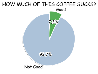
Finally, let’s finish getting our data ready for analysis by splitting it into training/test sets and standardizing the values to remove a bit of bias from the system.
#seperate feature/response vars
X = coffee.drop(columns=['goodCoffee'])
y = coffee['goodCoffee']
#train/test split
X_train, X_test, y_train, y_test = train_test_split(X, y, test_size=0.2, random_state=42)
#standardize values
sc = StandardScaler()
X_train = sc.fit_transform(X_train)
X_test = sc.transform(X_test)Test the Models
Random Forest Classifier
#better for mid-size datasets
rfc = RandomForestClassifier(n_estimators = 200)
rfc.fit(X_train, y_train)
pred_rfc = rfc.predict(X_test)
#how well did model perform?
print(classification_report(y_test, pred_rfc))
print(confusion_matrix(y_test, pred_rfc))precision recall f1-score support 0 0.98 0.98 0.98 244 1 0.74 0.74 0.74 19 accuracy 0.96 263 macro avg 0.86 0.86 0.86 263 weighted avg 0.96 0.96 0.96 263
SVM Classifier
#better for smaller datasets
clf = svm.SVC()
clf.fit(X_train, y_train)
pred_clf = clf.predict(X_test)
#how well did model perform?
print(classification_report(y_test, pred_clf))
print(confusion_matrix(y_test, pred_clf))precision recall f1-score support 0 0.98 0.98 0.98 244 1 0.78 0.74 0.76 19 accuracy 0.97 263 macro avg 0.88 0.86 0.87 263 weighted avg 0.97 0.97 0.97 263
Neural Network (Multi-Layer Percepitron Classifier)
#better for huge amounts of data
mlpc= MLPClassifier(hidden_layer_sizes=(11, 11, 11), max_iter=500)
mlpc.fit(X_train, y_train)
pred_mlpc = mlpc.predict(X_test)print(classification_report(y_test, pred_mlpc))
print(confusion_matrix(y_test, pred_mlpc))precision recall f1-score support 0 0.99 0.98 0.98 244 1 0.76 0.84 0.80 19 accuracy 0.97 263 macro avg 0.87 0.91 0.89 263 weighted avg 0.97 0.97 0.97 263
What’s Best?
from sklearn.metrics import accuracy_score
acc_rfc = accuracy_score(y_test, pred_rfc)
acc_clf = accuracy_score(y_test, pred_clf)
acc_mlpc = accuracy_score(y_test, pred_mlpc)

print(f"Random Forest was {acc_rfc:.2%} accurate")
print(f"SVM was {acc_clf:.2%} accurate")
print(f"Neural Network was {acc_mlpc:.2%} accurate")
Random Forest was 96.20% accurate
SVM was 96.58% accurate
Neural Network was 96.96% accurate
All our models preformed about the same, with the neural net just a little bit better than everyone else. We’ll implement that model. This is doubley nice because now we get to say “I implemented a neural network” which sounds very fancy indeed.
Predicting Future Values
#a reminder what our data looks like
coffee[90:100]| Aroma | Flavor | Aftertaste | Acidity | Body | Balance | goodCoffee | |
|---|---|---|---|---|---|---|---|
| 90 | 8.42 | 8.00 | 7.42 | 8.00 | 7.92 | 7.92 | 1 |
| 91 | 7.58 | 7.83 | 7.83 | 7.92 | 7.83 | 8.17 | 1 |
| 92 | 7.83 | 8.00 | 7.75 | 7.75 | 7.83 | 7.83 | 1 |
| 93 | 8.08 | 8.17 | 7.92 | 8.00 | 8.08 | 8.00 | 1 |
| 94 | 7.67 | 8.00 | 7.83 | 8.00 | 7.92 | 7.83 | 1 |
| 95 | 7.50 | 7.92 | 8.25 | 7.83 | 7.92 | 7.75 | 1 |
| 96 | 8.17 | 7.92 | 7.75 | 7.75 | 7.67 | 7.75 | 0 |
| 97 | 8.00 | 7.92 | 7.75 | 7.92 | 7.75 | 7.83 | 0 |
| 98 | 7.83 | 8.00 | 7.58 | 7.92 | 7.92 | 7.83 | 0 |
| 99 | 7.83 | 8.00 | 7.83 | 7.75 | 7.67 | 7.83 | 0 |
#---------------
#A theoretical cup of coffee
new_Aroma = 8
new_Flavor = 7.5
new_Aftertaste = 8
new_Acidity = 8
new_Body = 7.9
new_Balance = 8
#---------------
X_new = [[new_Aroma, new_Flavor, new_Aftertaste, new_Acidity, new_Body, new_Balance]]
X_new = sc.transform(X_new)
y_new = mlpc.predict(X_new)
print(y_new)
if y_new[0] == 1:
print("it's good!")
else:
print ("it's not good!")[1]
it's good!